Robust Calibration of Local Volatility Models
For the so-called local volatility model, Bruno Dupire derived a closed form solution, which, when naively applied, delivers cliffy volatility surfaces. A robust and fast parameter calibration scheme has to be found.
Problem overview
Call and/or put options on liquid assets or equity indices are traded for different expiries and for a range of strike prices. It turns out that the traded option prices do not fit into the constant volatility world of Black-Scholes but exhibit so-called “volatility smiles” or “volatility skewnesses”.
A model for which such a behavior can be obtained without the need of stochastic volatility is the local volatility model: Here the stochastic movement of the price of the underlying follows
$$dS = \mu S dt + \sigma(S,T) S\; dW$$
with the drift rate $\mu$, the volatility function $\sigma$ and the increment $dWdW$ of the Wiener process. The local volatility function cannot be measured directly, but has to be identified from the quoted option prices as mentioned above. Bruno Dupire showed in 1994: If these call prices were available as a function, then $\sigma$ must satisfy
$$
\sigma_\mathrm{loc}(K,T) = \sqrt{ \frac{ \frac{\partial C}{\partial T} + r K \frac{\partial C}{\partial K }} {\frac{K^2}{2} \frac{\partial^2 C}{\partial K^2}}}
$$
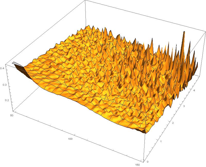
Function
When we apply this inversion formula directly, we obtain Local volatility surface by applying Dupire’s inversion formula on a 50×50 grid: Strikes from 50 to 150 percent of spot. Expiries up to 5 years. Synthetic implied (annual) volatilities between 25 and 35%. Noise level of up to absolute 0.1%.
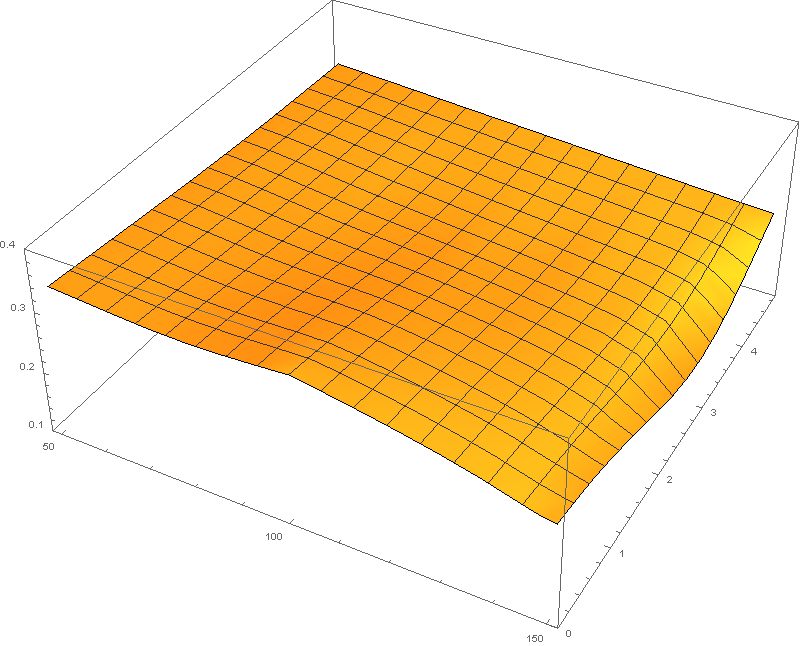
Model calibration example (synthetic data) – local volatility determined from call option prices, 0.01 % noise: